Manuscript for ICCFD12
Institute of Fluid Mechanics, Tsinghua University, Beijing, China
To solve a 2d conservation law (system)
\[\partial_{t}\,u+\partial_{\vec{r}}\vdot\vec{f}=0,\quad\partial_{\vec{r}}\vdot\vec{f}=\partial_{x}\,f^{x}+\partial_{y}\,f^{y},\]one first introduce a coordiante map
\[\underbrace{(x,y)}_{\vec{r}}\mapsto\underbrace{(\xi,\eta)}_{\vec{\rho}} \implies \begin{bmatrix}\partial_{\xi}\,\phi\\ \partial_{\eta}\,\phi \end{bmatrix}=\underbrace{\begin{bmatrix}\partial_{\xi}\,x & \partial_{\xi}\,y\\ \partial_{\eta}\,x & \partial_{\eta}\,y \end{bmatrix}}_{\underline{J}}\begin{bmatrix}\partial_{x}\,\phi\\ \partial_{y}\,\phi \end{bmatrix}=\begin{bmatrix}\partial_{\xi}\,\vec{r}\\ \partial_{\eta}\,\vec{r} \end{bmatrix}\vdot\partial_{\vec{r}}\,\phi,\]in which
\[U=u\,\underbrace{\det(\underline{J})}_{J},\quad\begin{bmatrix}F^{\xi}\\ F^{\eta} \end{bmatrix}=J\,\underbrace{\begin{bmatrix}\partial_{x}\,\xi & \partial_{y}\,\xi\\ \partial_{x}\,\eta & \partial_{y}\,\eta \end{bmatrix}}_{\underline{J}^{-1}}\begin{bmatrix}f^{x}\\ f^{y} \end{bmatrix}=J\begin{bmatrix}\partial_{\vec{r}}\,\xi\\ \partial_{\vec{r}}\,\eta \end{bmatrix}\vdot\vec{f}.\]Then, one might use either an orthonormal (modal) expansion or a Lagrange (nodal) interpolation for either \(u\) or \(U\equiv Ju\) on the \(j\)th element:
\[u(\vec{r},t)\approx u_{j}^{h}(\vec{r},t)=\begin{cases} \sum_{n=1}^{N}\hat{u}_{j,n}(t)\,\phi_{j,n}(\vec{\rho}), & \text{Lagrange interpolation},\\ \sum_{m=1}^{M}\tilde{u}_{j,m}(t)\,\psi_{j,m}(\vec{r}), & \text{orthonormal expansion}, \end{cases}\]A DG scheme might be formulated either in physical coordinates
\[\int_{E_j}\phi_n\pdv{u_j^h}{t} =\int_{E_j}\vec{f}_j^D\vdot\grad\phi_n -\oint_{\partial E_j}f^{I}\,\phi_n,\quad \forall n\in\{1,\dots,N\},\]or in parametric coordinates
\[\int_{\mathcal{E}_j}\phi_{n}\pdv{U_j^{h}}{t}=\int_{\mathcal{E}_j}\vec{F}_j^{D}\vdot\grad\phi_{n}-\oint_{\partial\mathcal{E}_j}F^{I}\,\phi_{n},\quad\forall n\in\{1,\dots,N\},\]A FR scheme is usually given in parametric coordinates
\[\begin{aligned}\dv{\hat{U}_{j,m,n}}{t} & =\frac{\partial F_{j}^{\xi,D}(\xi_{m},\eta_{n})}{\partial\xi}+\sum_{a=\pm1}\left[F^{I}-F_{j}^{\xi,D}\right]_{\xi=a,\eta_{n}}\dv{g_{a}(\xi_{m})}{\xi}\\ & +\frac{\partial F_{j}^{\eta,D}(\xi_{m},\eta_{n})}{\partial\eta}+\sum_{b=\pm1}\left[F^{I}-F_{j}^{\eta,D}\right]_{\xi_{m},\eta=b}\dv{g_{b}(\eta_{n})}{\eta}, \end{aligned}\]in which \(g\)’s are correction functions satisfying
\[g_{+1}(+1)=1,\quad g_{+1}(-1)=0,\quad g_{-1}(-\xi)=g_{+1}(+\xi),\quad \forall\xi\in[-1,1],\]and look like
| Typical Correction Functions |
|---|
 |
The original flux (disconstinuous on element interfaces) is reconstructed to be \(C_0\) constinuous in global:
| Flux Reconstruction Demo |
|---|
 |
Some choices of $g$ lead to the equivalent DG schemes:
| Equivalence between DG and FR |
|---|
 |
Common fluxes on element interfaces:
In this work, we use the last one (DDG):
\[\begin{bmatrix}\partial_{x}\,u\\ \partial_{y}\,u \end{bmatrix}_{\partial E}=\beta_{0}\,\Delta^{-1}\begin{bmatrix}n_{x}\,u\\ n_{y}\,u \end{bmatrix}_{\mathrm{R}-\mathrm{L}}+\begin{bmatrix}\partial_{x}\,u\\ \partial_{y}\,u \end{bmatrix}_{(\mathrm{R}+\mathrm{L})/2}+\beta_{1}\,\Delta \begin{bmatrix} n_x\,\partial^2_{xx}\,u + n_y\,\partial^2_{xy}\,u\\ n_x\,\partial^2_{yx}\,u + n_y\,\partial^2_{yy}\,u \end{bmatrix}_{\mathrm{R}-\mathrm{L}},\]⚠️ Physical derivatives from interpolations in parametric coordinates might be costly and error-prone.
If, the interpolation is applied to $u$, the second-order derivatives are
\[\begin{aligned}\begin{bmatrix}\partial_{xx}^{2}\,u & \partial_{xy}^{2}\,u\\ \partial_{yx}^{2}\,u & \partial_{yy}^{2}\,u \end{bmatrix} & =\underbrace{\underline{J}^{-1}\begin{bmatrix}\partial_{\xi}\\ \partial_{\eta} \end{bmatrix}}_{\begin{bmatrix}\partial_{x}\\ \partial_{y} \end{bmatrix}}\underbrace{\left(\mathinner{\begin{bmatrix}\partial_{\xi}\,u & \partial_{\eta}\,u\end{bmatrix}}\underline{J}^{-T}\right)}_{\begin{bmatrix}\partial_{x}\,u & \partial_{y}\,u\end{bmatrix}}\\ & =\underline{J}^{-1}\mathinner{\begin{bmatrix}\partial_{\xi}\mathinner{\begin{bmatrix}\partial_{\xi}\,u & \partial_{\eta}\,u\end{bmatrix}}\\ \partial_{\eta}\mathinner{\begin{bmatrix}\partial_{\xi}\,u & \partial_{\eta}\,u\end{bmatrix}} \end{bmatrix}}\underline{J}^{-T}+\underline{J}^{-1}\begin{bmatrix}\mathinner{\begin{bmatrix}\partial_{\xi}\,u & \partial_{\eta}\,u\end{bmatrix}}\partial_{\xi}\,\underline{J}^{-T}\\ \mathinner{\begin{bmatrix}\partial_{\xi}\,u & \partial_{\eta}\,u\end{bmatrix}}\partial_{\eta}\,\underline{J}^{-T} \end{bmatrix}, \end{aligned}\]in which the derivatives of the Jacobian matrix
\[\pdv{\underline{J}^{-T}}{\xi}=\left(-\underline{J}^{-1}\,\pdv{\underline{J}}{\xi}\,\underline{J}^{-1}\right)^{T},\quad \pdv{\underline{J}^{-T}}{\eta}=\left(-\underline{J}^{-1}\,\pdv{\underline{J}}{\eta}\,\underline{J}^{-1}\right)^{T},\]should be precomputed and cached on each flux point.
If the interpolation is applied to $U\equiv Ju$, the second-order derivatives are more complex:
\[\begin{aligned}\begin{bmatrix}\partial^2_{xx}\,u & \partial^2_{xy}\,u\\ \partial^2_{yx}\,u & \partial^2_{yy}\,u \end{bmatrix} & =\underbrace{\underline{J}^{-1}\begin{bmatrix}\partial_{\xi}\\ \partial_{\eta} \end{bmatrix}}_{\begin{bmatrix}\partial_{x}\\ \partial_{y} \end{bmatrix}}\underbrace{\left(\mathinner{\begin{bmatrix}\partial_{\xi}\,U & \partial_{\eta}\,U\end{bmatrix}}\underline{J}^{-T}\,J^{-1}-\mathinner{\begin{bmatrix}\partial_{\xi}\,J & \partial_{\eta}\,J\end{bmatrix}}\underline{J}^{-T}\,J^{-2}\,U\right)}_{\begin{bmatrix}\partial_{x}\,u & \partial_{y}\,u\end{bmatrix}}\\ & =\underline{J}^{-1}\mathinner{\begin{bmatrix}\partial_{\xi}\,\partial_{\xi}\,U & \partial_{\xi}\,\partial_{\eta}\,U\\ \partial_{\eta}\,\partial_{\xi}\,U & \partial_{\eta}\,\partial_{\eta}\,U \end{bmatrix}}\underline{J}^{-T}\,J^{-1}+\cdots, \end{aligned}\] \[\begin{aligned}\partial_{\xi}\left(\mathinner{\begin{bmatrix}\partial_{\xi}\,U & \partial_{\eta}\,U\end{bmatrix}}\underline{J}^{-T}\,J^{-1}\right) & =\mathinner{\begin{bmatrix}\partial_{\xi}\,\partial_{\xi}\,U & \partial_{\xi}\,\partial_{\eta}\,U\end{bmatrix}}\underline{J}^{-T}\,J^{-1}\\ & +\mathinner{\begin{bmatrix}\partial_{\xi}\,U & \partial_{\eta}\,U\end{bmatrix}}\left(\pdv{\underline{J}^{-T}}{\xi}\,J^{-1}+\underline{J}^{-T}\left(\partial_{\xi}\,J^{-1}\right)\right), \end{aligned}\] \[\begin{aligned}\partial_{\xi}\left(\mathinner{\begin{bmatrix}\partial_{\xi}\,J & \partial_{\eta}\,J\end{bmatrix}}\underline{J}^{-T}\,J^{-2}\,U\right) & =\mathinner{\begin{bmatrix}\partial_{\xi}\,\partial_{\xi}\,J & \partial_{\xi}\,\partial_{\eta}\,J\end{bmatrix}}\underline{J}^{-T}\,J^{-2}\,U\\ & +\mathinner{\begin{bmatrix}\partial_{\xi}\,J & \partial_{\eta}\,J\end{bmatrix}}\left(\pdv{\underline{J}^{-T}}{\xi}\,J^{-2}\,U+\underline{J}^{-T}\,\pdv{J^{-2}}{\xi}\,U+\underline{J}^{-T}\,J^{-2}\,\pdv{U}{\xi}\right), \end{aligned}\]in which, the derivatives of Jacobian determinant
\[\pdv{J^{-1}}{\xi}=-J^{-2}\,\pdv{J}{\xi},\quad\pdv{J^{-2}}{\xi}=-2J^{-3}\,\pdv{J}{\xi},\] \[\pdv{J}{\xi}=\pdv{\det(\underline{J})}{\xi}=\det(\underline{J})\tr(\underline{J}^{-1}\,\pdv{\underline{J}}{\xi})=J\tr(\underline{J}^{-1}\,\pdv{\underline{J}}{\xi}),\]should also be cached.
Take the scalar case in 1d space as an example:
\[\pdv{u}{t}+\pdv{f(u)}{x}=\pdv{x}\qty({\color{red}\nu(u)}\pdv{u}{x}),\quad \nu(u) \ge 0.\]Generalizing to systems:
\[\pdv{t}\mqty[u_1\\ \vdots \\ u_K]+\grad\vdot\mqty[\vb*{f}_1\\ \vdots \\ \vb*{f}_K] =\grad\vdot\mqty[{\color{red}\nu_1(u)}\grad{u}_1\\ \vdots \\ {\color{red}\nu_K(u)}\grad{u}_K],\]
For a one-dimensional system, the procedure could be applied to either each conservative variable or each characteristic variable.
For a multi-dimensional problem, we just apply the proposed procedure to each conservative variable, i.e.
Assume the viscosity value is a constant across the entire domain.
The semi-discretized ODE system can be written as
\[\dv{t}\ket{\hat{u}_{j}}=(\text{inviscid terms})+\nu\left(\underline{D}_{jj}\ket{\hat{u}_{j}}+\sum_{j'}\underline{D}_{jj'}\ket{\hat{u}_{j'}}\right),\]Without loss of generality, we hereforth only consider the nodal interpolation in which solution points are also Gaussian quadrature points.
One may now define the kinetic energy on $E_j$ to be
\[\begin{aligned} K_{j}\coloneqq\int_{E_{j}}\frac{1}{2}\qty(u_{j}^{h})^{2} &\approx\frac{1}{2}\sum_{n=1}^{N}w_{j,n}\,\hat{u}_{j,n}\,\hat{u}_{j,n} \\ &=\frac{1}{2}\underbrace{\begin{bmatrix}\hat{u}_{j,1} & \cdots & \hat{u}_{j,N}\end{bmatrix}}_{\bra{\hat{u}_{j}}}\underbrace{\begin{bmatrix}w_{j,1}\\ & \ddots\\ & & w_{j,N} \end{bmatrix}}_{\underline{W}_{j}}\underbrace{\begin{bmatrix}\hat{u}_{j,1}\\ \vdots\\ \hat{u}_{j,N} \end{bmatrix}}_{\ket{\hat{u}_{j}}}, \end{aligned}\]The dissipation rate of $K_j$ can easily be derived, which is
\[\begin{aligned} \dv{K_j}{t} &=\bra{\hat{u}_{j}}\underline{W}_{j}\dv{t}\ket{\hat{u}_{j}} \\ &=(\text{inviscid terms})+\nu\,\underbrace{\bra{\hat{u}_{j}}\underline{W}_{j}\,\underline{D}_{jj}\ket{\hat{u}_{j}}}_{G_j}+(\text{inter-cell viscous terms}), \end{aligned}\]By ignoring the inviscid terms and inter-cell viscous terms, one gets
\[\nu_{j}=\frac{\Delta K_{j}}{-G_{j}\,\tau_j} \impliedby\dv{t}K_{j}=\cdots+\nu\,G_{j}+\cdots,\]in which
\[\tau_j = C \frac{h_j}{\lambda_\max},\]\(C\) is the only tuneable parameter.
⚠️ To avoid extremely large viscosity:
\[\nu_{j}=\min\qty(\frac{-\Delta K_{j}}{G_{j}\cdot\tau_j},\lambda_\max\frac{h_j}{P}),\]⚠️ To avoid 0-in-divisor:
| Large \(\nu\) caused by \(0\)-in-divisor |
|---|
 |
The last question is how to evaluate the oscillation energy $\Delta K_j$, which quantitatively measures the numerical oscillation on $E_j$.
In one-dimensional cases, we define it to be
\[\Delta K_j = \int_{x_{j-1/2}}^{x_{j}}\left(u_{j}^{h}-u_{j-1}^{h}\right)^{2}\dd{x}+\int_{x_{j}}^{x_{j+1/2}}\left(u_{j}^{h}-u_{j+1}^{h}\right)^{2}\dd{x},\]Both the integrals and extrapolations are cheap.
However, when it is generalized to multi-dimensional cases, one has to (iteratively) solve
\[\mqty[x \\ y]_\text{query} = \mqty[x^h(\xi, \eta) \\ y^h(\xi, \eta)],\]for the value of $(\xi,\eta)$ from the given $(x,y)$ on a neighboring cell.
Even worse, the solution of this equation might not exist:
| Failed Coordinate Map |
|---|
 |
In the current work, we use the following surface integral of value jumps
\[\oint_{\partial E_j} \qty(u^h_{j}-u^h_{j'})^2,\quad j'\in\text{ neighbors of } E_j,\]which is a simplified case of the one used in variational reconstruction.
Further tests on more challenging problems are still in progress.
It is an open problem to design an oscillation measure requiring no extrapolations.
Common settings:
Additional common settings:
| Density | Viscosity |
|---|---|
 |  |
| Density | Viscosity |
|---|---|
 |  |
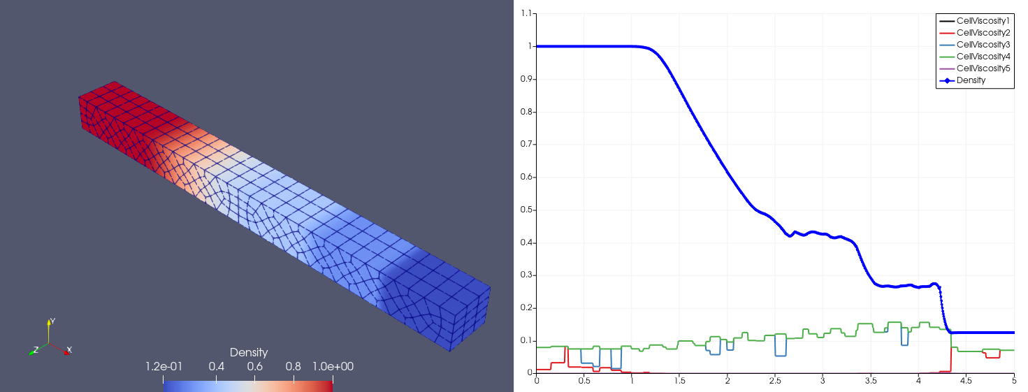
Proposed by Shu (1989)
\[\mqty[\rho & u & p]_{t=0} = \begin{cases} \mqty[3.857143 & 2.629369 & 10.33333], &x\in[0,1);\\ \mqty[1+0.2\sin(5x) & 0 & 1], &x\in(1,10]. \end{cases}\]| Density | Viscosity |
|---|---|
 |  |
| \(P=2\) | \(P=3\) | |
|---|---|---|
| \(N_x=25\) |  |  |
| \(N_x=100\) |  |  |
Lax (1997) defines dozens of 2D Riemann problems.
The one we solve is
\[\begin{bmatrix}\rho \\ u \\ v \\ p\end{bmatrix}_{t=0}=\begin{cases} \begin{bmatrix}1.5 & 0 & 0 & 1.5\end{bmatrix}^T, & (x,y)\in(0.8,1)\times(0.8,1),\\ \begin{bmatrix}0.5323 & 1.206 & 0 & 0.3\end{bmatrix}^T, & (x,y)\in(0,0.8)\times(0.8,1),\\ \begin{bmatrix}0.138 & 1.206 & 1.206 & 0.029\end{bmatrix}^T, & (x,y)\in(0,0.8)\times(0,0.8),\\ \begin{bmatrix}0.5323 & 0 & 1.206 & 0.3\end{bmatrix}^T, & (x,y)\in(0.8,1)\times(0,0.8), \end{cases}\]Two shocks interfere with each other:
| \(P=2\) | \(P=3\) | |
|---|---|---|
| \(h=0.05\) |  |  |
| \(h=0.01\) |  |  |
Proposed by Woodward (1984)
| Sketch of the Double Mach Reflection Problem |
|---|
 |
\(h\approx 0.02\), \(P=2\) with the simple compact WENO limiter:
| Reference Solution Given by Limiter |
|---|
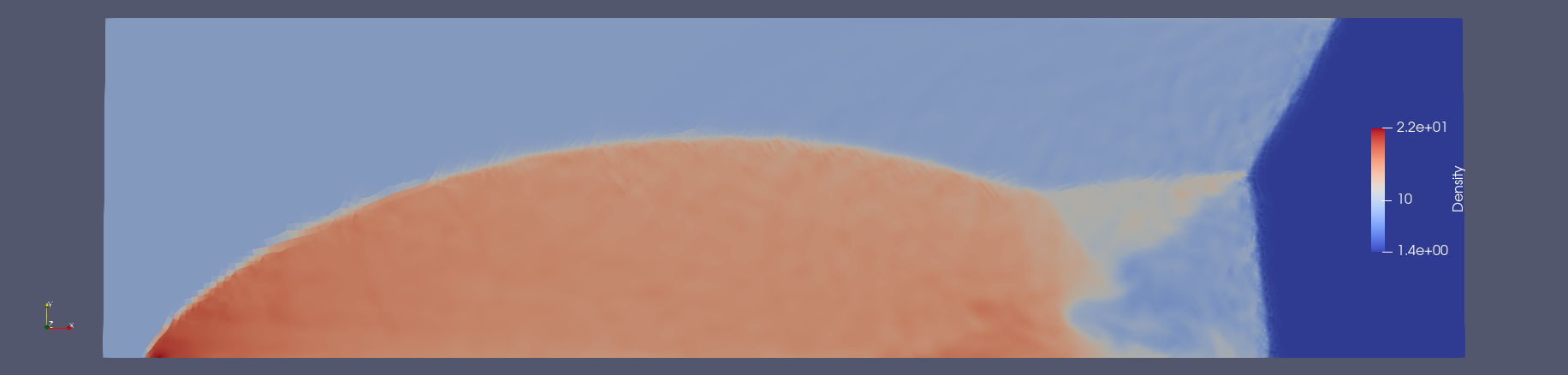 |
\(h\approx 0.05\) by the proposed artificial viscosity:
| \(P\) | Value | \(t=0.8\) |
|---|---|---|
| 2 | \(\rho(t=0.25)\) |  |
| 3 | \(\rho(t=0.25)\) | 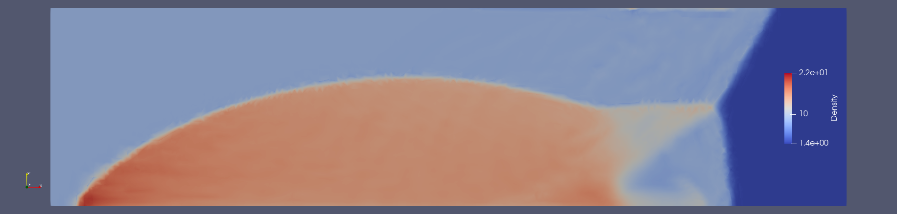 |
| 3 | \(\nu\) for \(\rho(t=0.25)\) | 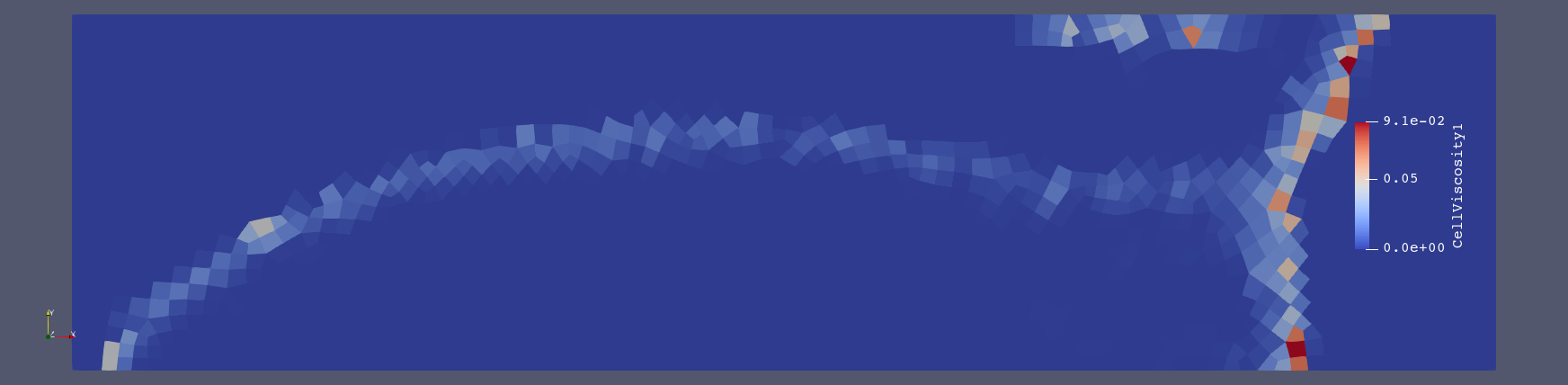 |
| 3 | \(\nu\) for \(\rho v(t=0.25)\) | 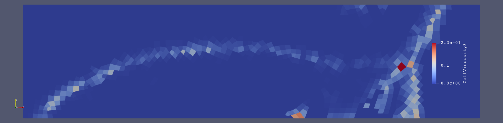 |
| 3 | \(\rho v(t=0.25)\) | 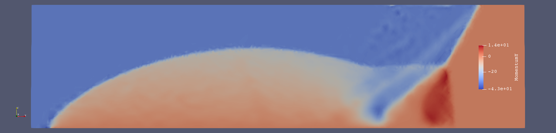 |
The proposed artificial viscosity
Further improvements might include